
Airport market share by ZIP code measures the percentage of air travelers living in a ZIP code who choose a particular airport for their trips.
The basic calculation is:
Airport Market Share = Passengers from the ZIP Code Using the Airport ÷ Total Air Passengers from the ZIP Code × 100
For example, if residents of a ZIP code generate an estimated 20,000 annual air passenger trips and 8,000 of those trips use Airport A, Airport A’s market share in that ZIP code is:
8,000 ÷ 20,000 = 40%
Calculating market share at the ZIP-code level gives airports a detailed geographic view of their position across the region and can reveal patterns that are hidden by airport-wide or catchment-wide averages.
What Does Airport Market Share by ZIP Code Tell You?
Airport market share answers a different question from passenger volume.
Passenger volume answers:
“How many of our passengers live in this ZIP code?”
Market share answers:
“Of all the air travelers living in this ZIP code, what percentage use our airport?”
Consider two ZIP codes:
| ZIP Code | Total Air Passenger Demand | Passengers Using Airport A | Airport A Market Share |
|---|---|---|---|
| ZIP A | 10,000 | 7,000 | 70% |
| ZIP B | 30,000 | 12,000 | 40% |
Airport A receives more passengers from ZIP B—12,000 compared with 7,000.
But Airport A has a much stronger market position in ZIP A, where it captures 70% of total air travel demand.
Passenger volume measures contribution to the airport. Market share measures the airport’s position within the local market.
Step 1: Estimate Total Air Travel Demand from the ZIP Code
The denominator is critical.
To calculate airport market share correctly, you first need an estimate of the total air passenger demand generated by residents of the ZIP code, regardless of which airport they use.
Suppose ZIP 22030 generates:
25,000 resident air passenger trips per year
Those passengers may use several airports:
| Airport | Resident Passenger Trips |
| Airport A | 11,250 |
| Airport B | 7,500 |
| Airport C | 5,000 |
| Other airports | 1,250 |
| Total | 25,000 |
Step 2: Estimate Which Airport Those Passengers Use
The next step is to distribute the ZIP code’s passenger demand among the airports residents actually use.
Using the example above:
- Airport A: 11,250 ÷ 25,000 = 45%
- Airport B: 7,500 ÷ 25,000 = 30%
- Airport C: 5,000 ÷ 25,000 = 20%
- Other airports: 1,250 ÷ 25,000 = 5%
Airport A therefore has a 45% market share of resident air passenger demand in this ZIP code.
Importantly, market share does not require assigning the ZIP code exclusively to one airport. Multiple airports can—and usually do—serve passengers from the same ZIP code.
Step 3: Repeat the Calculation Across ZIP Codes
The real value comes from repeating the calculation across the airport’s broader market.
The results might look like:
| ZIP Code | Total Demand | Airport Passengers | Airport Market Share |
| ZIP A | 12,000 | 9,600 | 80% |
| ZIP B | 18,000 | 11,700 | 65% |
| ZIP C | 25,000 | 12,500 | 50% |
| ZIP D | 30,000 | 10,500 | 35% |
| ZIP E | 20,000 | 4,000 | 20% |
When these values are mapped, the airport’s geographic market position becomes much easier to see.
Instead of drawing a single catchment boundary, an airport can see how its share changes from community to community.
Airport Market Share Is Not the Same as Share of Airport Passengers
These two measures are easy to confuse.
Suppose an airport handles 500,000 resident passenger trips annually and 25,000 come from ZIP A.
ZIP A therefore contributes:
25,000 ÷ 500,000 = 5% of the airport’s resident passengers.
But suppose ZIP A generates 40,000 total air passenger trips across all airports.
The airport’s market share within ZIP A is:
25,000 ÷ 40,000 = 62.5%.
So:
5% = ZIP A’s contribution to the airport
while
62.5% = the airport’s share of ZIP A
They describe completely different relationships.
For catchment and geographic market analysis, airport share of the ZIP code is generally the relevant measure.
Why ZIP-Level Market Share Is More Useful Than One Overall Percentage
Suppose an airport captures 45% of passenger demand across its entire study area.
That single number provides a useful summary, but it does not show where the airport is strong or weak.
The underlying geography might look like:
- Nearby ZIP codes: 70–85% market share
- Middle ZIP codes: 45–65%
- Outer ZIP codes: 20–40%
A catchment-wide average of 45% hides all of this variation.
ZIP-level analysis reveals the spatial structure behind the overall result.
This is particularly useful for airports serving large metropolitan regions or areas where several commercial airports are accessible.
Real-World Example: Harrisburg International Airport
Harrisburg International Airport (MDT) has been the subject of academic research specifically examining airport catchment behavior at the ZIP-code level.
Researchers constructed a ZIP-code spatial database of airport customers to analyze MDT’s market area in south-central Pennsylvania. The analysis found clear geographic patterns in airport substitution, particularly between Harrisburg and Baltimore/Washington International Airport (BWI).
This is exactly the type of pattern that a single regional market-share figure can obscure.
One ZIP code may have a strong MDT position, while another ZIP code farther south or closer to major transportation corridors may show a very different distribution of airport use.
The Harrisburg example demonstrates why airport market position is inherently geographic and why ZIP-level analysis can provide more insight than treating an entire catchment as one homogeneous market.
Real-World Example: Hagerstown’s Multi-Airport Market
Hagerstown Regional Airport (HGR) provides an especially clear example of why the denominator needs to include travelers using all relevant airports.
A 2023 catchment study covering a 44-ZIP-code immediate market estimated approximately 902,938 domestic airline trips.
Those trips were distributed heavily among Washington-Baltimore area airports:
- BWI: 44.3%
- IAD: 29.3%
- DCA: 17.8%
Other airports accounted for smaller portions of the market.
This demonstrates that residents of a geographic area can distribute their trips across several airports.
A ZIP-level calculation takes the same concept one step further: instead of calculating one share for all 44 ZIP codes combined, the calculation is performed separately for each ZIP code.
That can show where BWI’s share is strongest, where IAD becomes more important, where DCA attracts meaningful demand, and how airport-choice patterns transition across the region.
Market Share Can Also Be Calculated by Destination
Overall ZIP-code market share is useful, but Air Service Development teams may also want to calculate market share for an individual destination.
The calculation becomes:
Airport Destination Market Share = ZIP-to-Destination Passengers Using the Airport ÷ Total ZIP-to-Destination Passengers Using All Airports
For example, suppose residents of one ZIP code generate 1,000 annual passenger trips to Orlando:
- Airport A: 650 passengers
- Airport B: 250 passengers
- Airport C: 100 passengers
Airport A has a 65% share of the ZIP code’s Orlando market.
But the same airport might have only a 35% share for Los Angeles.
This distinction can be valuable for route development because an airport’s geographic strength may vary significantly by destination.
Market Share Can Be Calculated for Different Passenger Segments
The same framework can also be applied to different passenger populations.
For example, airports may analyze market share for:
- All resident passengers
- Premium passengers
- Domestic passengers
- International passengers
- Specific destinations
- Specific time periods
A ZIP code where an airport captures 50% of all resident passengers could have a very different share among premium or international travelers.
Segmenting the calculation helps airport teams understand where their market position differs from the overall average.
Why the Time Period Matters
Market share should always be associated with a defined time period.
Airline schedules change. New routes begin. Routes are discontinued. Fares change. Passenger behavior evolves.
An airport might have: 42% market share in 2024 and 48% market share in 2026 in the same ZIP code.
Tracking ZIP-level market share over time can reveal whether the airport’s geographic position is strengthening, weakening, or remaining stable.
It can also help identify where changes are occurring rather than relying only on an airport-wide trend.
How Fligence Can Show Airport Market Share by ZIP Code
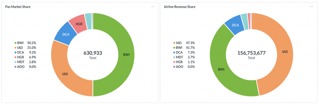
FlightBI’s Fligence passenger-location analysis estimates resident air passenger demand at the ZIP-code level and identifies the airports those travelers use.
This allows airport teams to compare:
Total resident air travel demand from each ZIP code
with
Resident passenger demand using the target airport
to calculate the airport’s ZIP-level market share.
The results can then be viewed geographically, as the platform allows users to group ZIP codes, making it easier to see how airport position varies across the region.
For each ZIP code or ZIP group, the fundamental question becomes:
“Of all resident air travelers from this ZIP code/group, what percentage use our airport?”
That provides a much more actionable geographic measure than simply counting how many airport passengers live there.
How Air Service Development Teams Can Use ZIP-Level Market Share
For Air Service Development teams, ZIP-level market share can provide a more detailed picture of the airport’s geographic strength.
It can help teams:
- Quantify the airport’s position across its broader market
- Demonstrate strong geographic areas in airline presentations
- Identify how market position changes across the catchment
- Compare overall and destination-specific market share
- Track geographic changes over time
- Support estimates of the airport’s addressable passenger market
- Analyze passenger segments separately
It can also provide important context when evaluating a proposed route.
If a destination has substantial passenger demand in ZIP codes where the airport already has a strong position, that may tell a different story from demand concentrated in areas where the airport has a relatively small share.
How Airport Marketing Teams Can Use ZIP-Level Market Share
For airport marketing teams, market share adds important context to passenger-volume maps.
A ZIP code generating many airport passengers may already be a very strong market.
Another ZIP code may generate fewer airport passengers but contain much greater total air travel demand.
Looking at passenger volume and market share together helps distinguish different types of geographic markets and can support more informed decisions about where to conduct further marketing analysis.
The key is not to assume that the ZIP code with the most current passengers is automatically the ZIP code with the greatest opportunity.
Data Quality Matters
ZIP-level market share is only as reliable as the passenger-location and airport-choice data behind it.
Historically, airports often relied on passenger surveys to estimate where travelers lived. Today, mobile-location and other digital datasets can provide much larger samples, but those datasets also require careful calibration.
For example, raw mobile-location observations may not represent all passenger populations equally, and the number of observed devices should not automatically be treated as actual passenger volume.
A robust methodology should therefore reconcile geographic passenger observations with aviation demand data before calculating market share.
The objective is not simply to count observed devices. It is to estimate actual passenger demand and airport choice at the ZIP-code level.
The Bottom Line
Airport market share by ZIP code is calculated by dividing the number of passengers from a ZIP code who use the target airport by the total number of air passengers generated by that ZIP code across all relevant airports.
The calculation is simple:
Airport passengers from ZIP ÷ Total air passengers from ZIP × 100
The challenge is obtaining reliable estimates for both parts of that equation.
Once calculated across an airport’s market, ZIP-level market share provides a detailed geographic picture of airport position that cannot be seen from airport traffic totals or a single catchment-wide percentage.
It tells airport teams not only where their passengers live, but how strong the airport’s position is within each local market.